pathfindR is an R package for pathway/gene-set enrichment analysis that does something most enrichment tools don’t: instead of testing your gene list directly, it first maps your genes onto a protein–protein interaction network (PIN), finds active subnetworks (connected groups of interacting genes that are enriched for significantly altered genes), and then runs enrichment on those subnetworks. The payoff is that genes which don’t pass your significance cutoff on their own (but sit in the middle of a cluster of genes that do) still get a chance to contribute.
This post walks through a typical workflow end to end: run the analysis, cluster the results, visualize, and score terms per sample.
What changed in 3.0.0: no more Java
If you used older versions, you’ll remember the asterisk next to “easy install”:
the active subnetwork search ran on a bundled Java .jar, so you needed a JRE on
your PATH and a fair amount of “is Java configured correctly?” troubleshooting.
As of pathfindR 3.0.0, that’s gone. The greedy (GR), simulated annealing (SA), and genetic (GA) search algorithms have been re-implemented in R and C++ (via Rcpp), and the Java dependency was removed entirely. For GR and SA, results are numerically identical to the legacy JAR given the same seed and inputs so this is a drop-in upgrade, not a behaviour change. Installation is now just:
install.packages("pathfindR")
That’s the whole story. No JAVA_HOME, no PATH surgery.
The input
The input is a simple data frame with three columns: a gene symbol, an
(optional) change value such as log-fold-change, and a p-value. pathfindR ships
with an example derived from a rheumatoid arthritis vs. healthy
differential-expression dataset (GEO GSE15573):
library(pathfindR)
#> Loading required package: pathfindR.data

head(example_pathfindR_input)
#>   Gene.symbol    logFC  adj.P.Val
#> 1     FAM110A -0.69394 3.4087e-06
#> 2      RNASE2  1.35350 1.0085e-05
#> 3      S100A8  1.54483 3.4664e-05
#> 4      S100A9  1.02809 2.2626e-04
#> 5      TEX261 -0.32360 2.2626e-04
#> 6    ARHGAP17 -0.69193 2.7081e-04
Running the analysis
The wrapper run_pathfindR() takes you from input to enriched terms in one call:
it processes the input, maps it onto the PIN, searches for active subnetworks,
and runs enrichment over a chosen number of iterations.
output_df <- run_pathfindR(example_pathfindR_input)
A few arguments worth knowing (all optional):
# pick the gene sets (default = "KEGG")
output_df <- run_pathfindR(example_pathfindR_input, gene_sets = "GO-MF")

# pick the PIN for the subnetwork search (default = "Biogrid")
output_df <- run_pathfindR(example_pathfindR_input, pin_name_path = "STRING")

# write the HTML report somewhere specific
output_df <- run_pathfindR(example_pathfindR_input, output_dir = "RA_results")
Available PINs include "Biogrid", "STRING", "GeneMania", "IntAct",
"KEGG" and "mmu_STRING"; available gene sets include "KEGG", "Reactome",
"BioCarta", the GO families ("GO-All", "GO-BP", "GO-CC", "GO-MF") and
"mmu_KEGG". You can also supply a custom PIN or custom gene sets.
The result is a data frame, one row per enriched term, with the term ID and description, enrichment p-values (lowest/highest across iterations), fold enrichment, and the affected up-/down-regulated input genes. The package also bundles a pre-computed copy of this output so we can keep going without waiting on the search:
head(example_pathfindR_output, 4)
#>         ID                          Term_Description Fold_Enrichment occurrence
#> 1 hsa05415                   Diabetic cardiomyopathy          3.7450         10
#> 2 hsa03082        ATP-dependent chromatin remodeling          4.2131         10
#> 3 hsa04130 SNARE interactions in vesicular transport          4.9366         10
#> 4 hsa00190                 Oxidative phosphorylation          3.5587         10
#>    support   lowest_p  highest_p
#> 1 0.087103 4.1728e-15 1.1843e-08
#> 2 0.024579 1.8507e-12 3.1203e-04
#> 3 0.033857 2.8509e-09 8.7854e-09
#> 4 0.044888 4.1980e-09 4.3382e-06
#>                                                      Up_regulated
#> 1 NCF4, NDUFA1, NDUFB3, UQCRQ, COX6A1, COX7A2, COX7C, MMP9, GAPDH
#> 2
#> 3                                                            STX6
#> 4 NDUFB3, NDUFA1, COX7C, COX7A2, UQCRQ, COX6A1, ATP6V1D, ATP6V0E1
#>                                                  Down_regulated
#> 1              SLC25A5, VDAC1, ATP2A2, MTOR, PDHA1, PDHB, PARP1
#> 2 ARID1A, SMARCA4, ACTB, ACTG1, BRD7, BRD9, HDAC1, EP400, TRRAP
#> 3                                           BET1L, SNAP23, STX2
#> 4                                                      ATP6V0E2
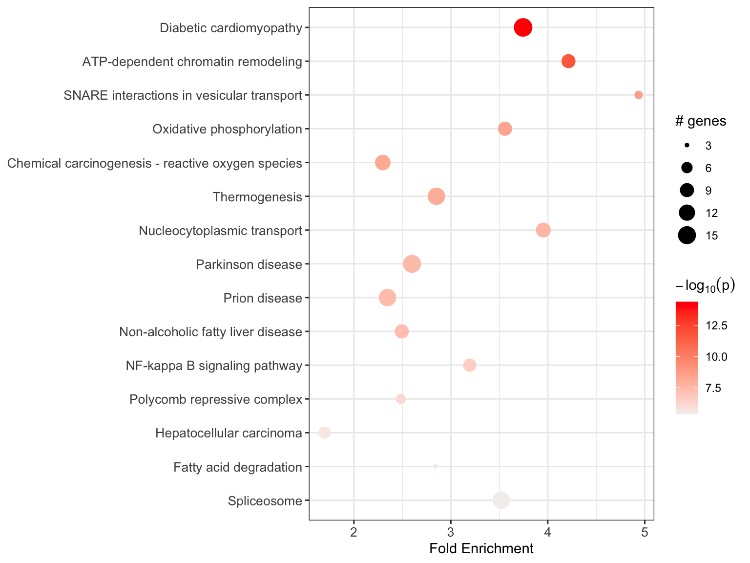
A quick way to eyeball the top hits is the enrichment chart, a bubble plot of the most significant terms:
enrichment_chart(example_pathfindR_output, top_terms = 15)
#> Plotting the enrichment bubble chart
Clustering the enriched terms
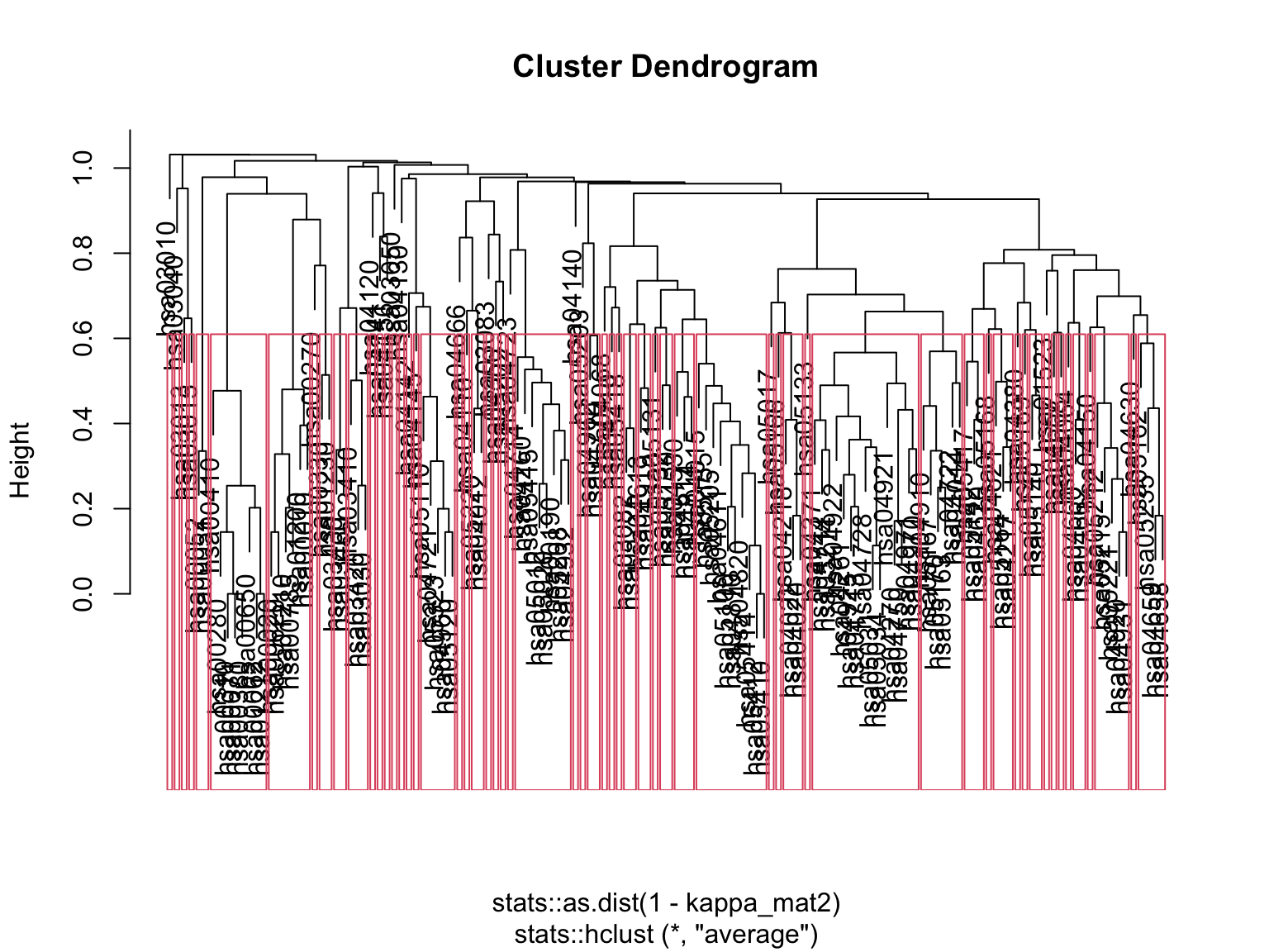
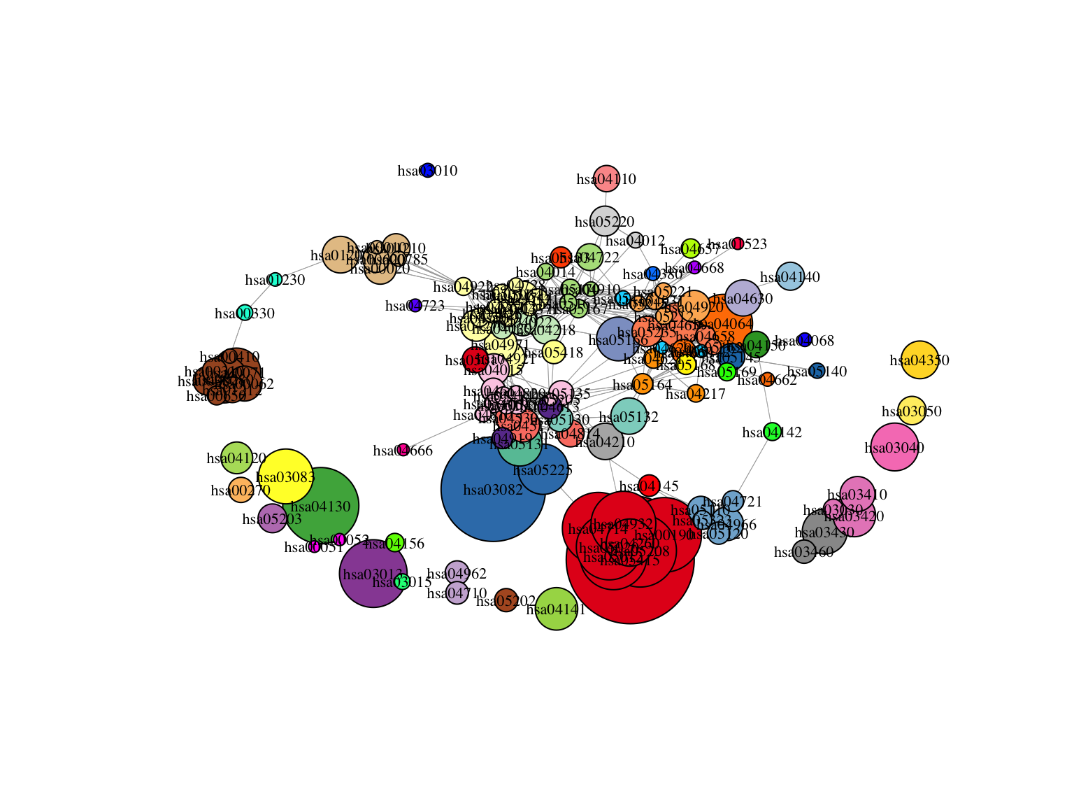
Enrichment output is often redundant, several terms describe overlapping
biology. cluster_enriched_terms() computes pairwise kappa statistics between
terms, clusters them (hierarchical by default), picks the cluster count that
maximizes the average silhouette width, and tags one representative term per
cluster:
clustered_df <- cluster_enriched_terms(example_pathfindR_output)
#> The maximum average silhouette width was 0.24 for k = 60
# the representative term from each cluster
clustered_df[clustered_df$Status == "Representative", c("Term_Description", "Cluster")]
#>                                       Term_Description Cluster
#> 1                              Diabetic cardiomyopathy       1
#> 2                   ATP-dependent chromatin remodeling       2
#> 3            SNARE interactions in vesicular transport       3
#> 7                          Nucleocytoplasmic transport       4
#> 11                        NF-kappa B signaling pathway       5
#> 12                         Polycomb repressive complex       6
#> 14                              Fatty acid degradation       7
#> 15                                         Spliceosome       8
#> 18                                     Mismatch repair       9
#> 19                                         Shigellosis      10
#> 20                           Th17 cell differentiation      11
#> 21             Human T-cell leukemia virus 1 infection      12
#> 22                          Nucleotide excision repair      13
#> 23         Protein processing in endoplasmic reticulum      14
#> 24                          TGF-beta signaling pathway      15
#> 25                                   Carbon metabolism      16
#> 26                                           Apoptosis      17
#> 27                                Salmonella infection      18
#> 28                          Oxytocin signaling pathway      19
#> 29                          JAK-STAT signaling pathway      20
#> 32                                  IgSF CAM signaling      21
#> 33                      Collecting duct acid secretion      22
#> 37                     Adipocytokine signaling pathway      23
#> 38                      Ubiquitin mediated proteolysis      24
#> 40                              Rap1 signaling pathway      25
#> 42                            Chronic myeloid leukemia      26
#> 44                                Viral carcinogenesis      27
#> 45                                 Cellular senescence      28
#> 46                                          Proteasome      29
#> 47                                  Autophagy - animal      30
#> 51                                       Toxoplasmosis      31
#> 52                      Neurotrophin signaling pathway      32
#> 55                              mTOR signaling pathway      33
#> 56                                          Cell cycle      34
#> 57                              Spinocerebellar ataxia      35
#> 61                  Cysteine and methionine metabolism      36
#> 64                   T cell receptor signaling pathway      37
#> 65            Vasopressin-regulated water reabsorption      38
#> 66             Neutrophil extracellular trap formation      39
#> 68              Fluid shear stress and atherosclerosis      40
#> 70             Transcriptional misregulation in cancer      41
#> 73                                        Phagocytosis      42
#> 77                                           Pertussis      43
#> 79                                         Influenza A      44
#> 81                    Herpes simplex virus 1 infection      45
#> 86                             IL-17 signaling pathway      46
#> 92  Integrated stress response (ISR) signaling pathway      47
#> 97                        Epstein-Barr virus infection      48
#> 99                                 Lysosome biogenesis      49
#> 111                          mRNA surveillance pathway      50
#> 114                    Arginine and proline metabolism      51
#> 118                          Lipid and atherosclerosis      52
#> 123                         Osteoclast differentiation      53
#> 124                                           Ribosome      54
#> 126                             FoxO signaling pathway      55
#> 131               Retrograde endocannabinoid signaling      56
#> 132                              TNF signaling pathway      57
#> 134                               Galactose metabolism      58
#> 136            Fc gamma R-mediated phagosome formation      59
#> 137                              Antifolate resistance      60

enrichment_chart(example_pathfindR_output, plot_by_cluster = TRUE)
#> Plotting the enrichment bubble chart
#> For plotting by cluster, there must a column named `Cluster` in the input data frame!
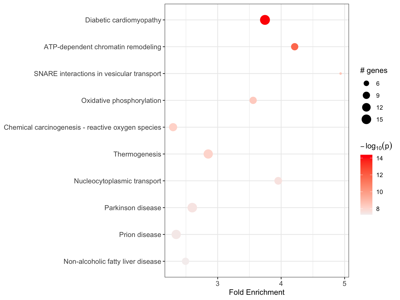
Filtering to representatives gives you a compact, non-redundant shortlist to
report. There’s also a method = "fuzzy" option if you’d rather let terms belong
to more than one cluster.
Visualizing results
Beyond the enrichment chart, two visuals are especially handy.
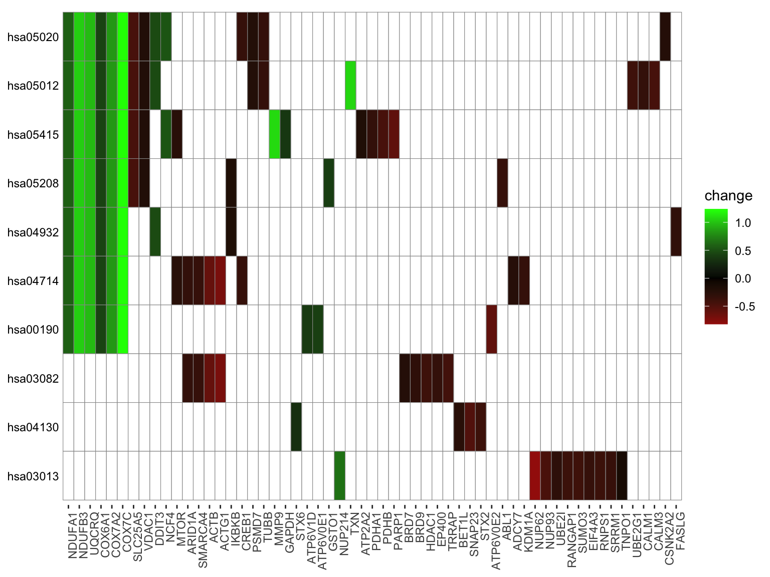
A term–gene heatmap shows which input genes drive which terms. If you pass the original input, tiles are colored by change value:
term_gene_heatmap(example_pathfindR_output, example_pathfindR_input, num_terms = 10)
#> ## Processing input. Converting gene symbols,
#>           if necessary (and if human gene symbols provided)
#> Number of genes provided in input: 572
#> Number of genes in input after p-value filtering: 572
#>
#> Could not find any interactions for 1 (0.17%) genes in the PIN
#> Final number of genes in input: 571
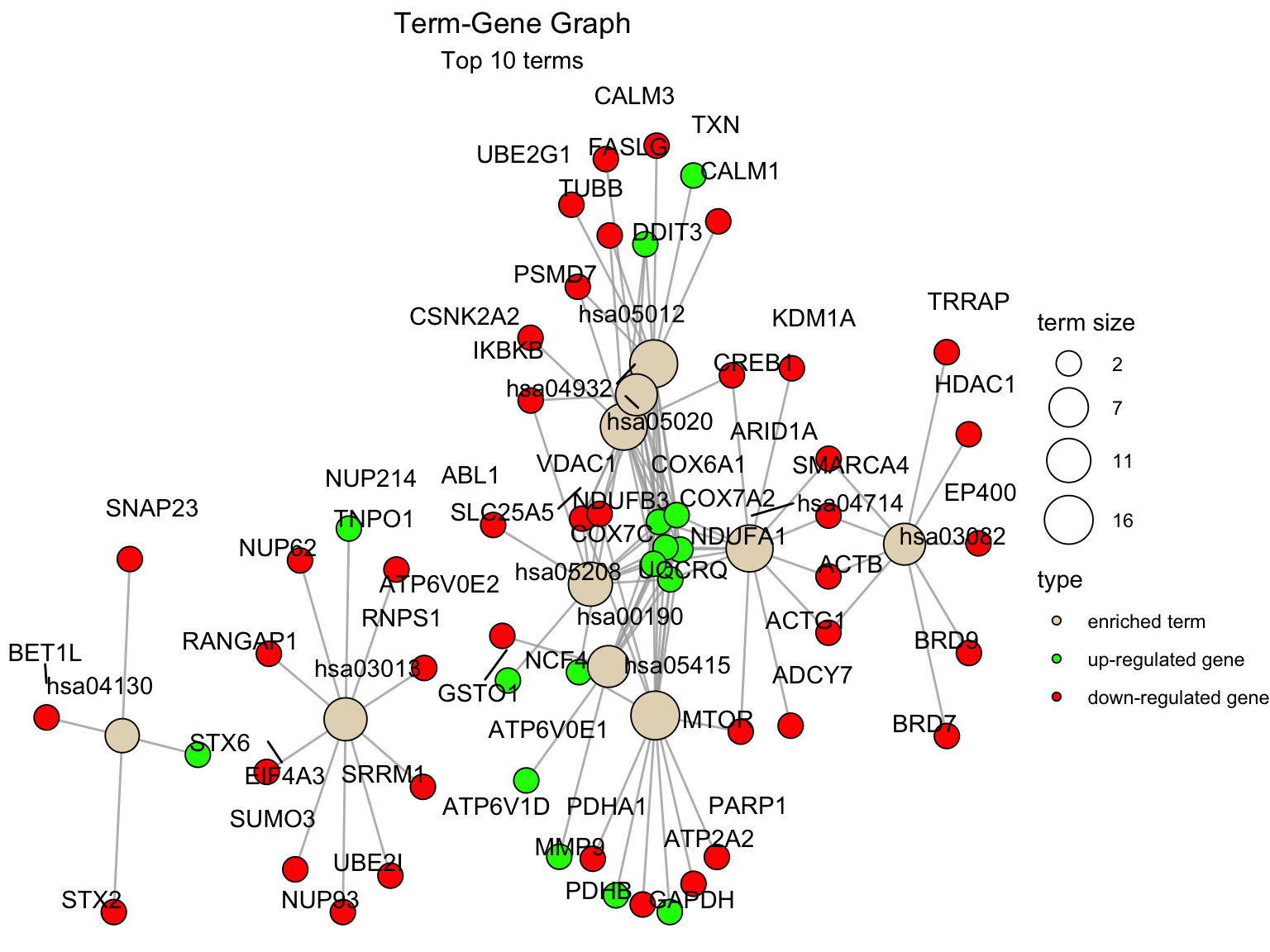
A term–gene graph shows the same relationships as a network, making shared genes between terms obvious. As of 3.x this is split into a builder and a plotter:
g <- create_term_gene_graph(example_pathfindR_output, num_terms = 10)
create_term_gene_plot(g)
Scoring terms per sample
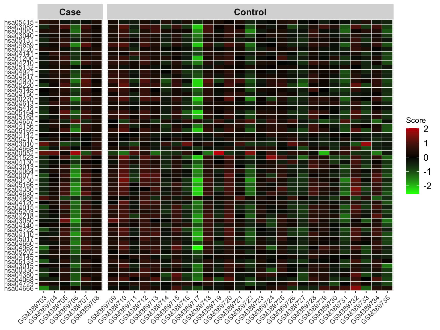
If you have a per-sample expression matrix, score_terms() computes an
agglomerated z-score for each enriched term in each sample — useful for seeing
whether a pathway is collectively activated or repressed in particular samples or
groups:
case_sample_ids <- c(
  "GSM389703", "GSM389704", "GSM389705", "GSM389706", "GSM389707", "GSM389708"
)
score_matrix <- score_terms(
  enrichment_table = clustered_df[clustered_df$Status == "Representative", ],
  exp_mat          = example_experiment_matrix,   # genes x samples
  cases            = case_sample_ids,             # optional
  plot_hmap        = TRUE
)
Putting it together
The whole everyday workflow is really just:
library(pathfindR)

output_df    <- run_pathfindR(example_pathfindR_input)          # enrichment
clustered_df <- cluster_enriched_terms(output_df)               # de-duplicate
enrichment_chart(clustered_df, plot_by_cluster=TRUE)            # visualize
term_gene_heatmap(output_df, example_pathfindR_input)           # who drives what
Four functions, and no Java to install. If you’re comparing two
conditions, take a look at combine_pathfindR_results() too.
pathfindR is described in Ulgen E, Ozisik O, Sezerman OU. 2019. pathfindR: An R Package for Comprehensive Identification of Enriched Pathways in Omics Data Through Active Subnetworks. Front. Genet. https://doi.org/10.3389/fgene.2019.00858. Docs: https://egeulgen.github.io/pathfindR/.