Introduction to pathfindR

pathfindR is a tool for enrichment analysis via active subnetworks. The package also offers functionality to cluster the enriched terms and identify representative terms in each cluster, to score the enriched terms per sample and to visualize analysis results.

The functionality suite of pathfindR is described in detail in Ulgen E, Ozisik O, Sezerman OU. 2019. pathfindR: An R Package for Comprehensive Identification of Enriched Pathways in Omics Data Through Active Subnetworks. Front. Genet. https://doi.org/10.3389/fgene.2019.00858

Overview

The observation that motivated us to develop pathfindR was that direct enrichment analysis of differential RNA/protein expression or DNA methylation results may not provide the researcher with the full picture. That is to say: enrichment analysis of only a list of significant genes alone may not be informative enough to explain the underlying disease mechanisms. Therefore, we considered leveraging interaction information from a protein-protein interaction network (PIN) to identify distinct active subnetworks and then perform enrichment analyses on these subnetworks.

An active subnetwork can be defined as a group of interconnected genes in a PIN that predominantly consists of significantly altered genes. In other words, active subnetworks define distinct disease-associated sets of interacting genes, whether discovered through the original analysis or discovered because of being in interaction with a significant gene.

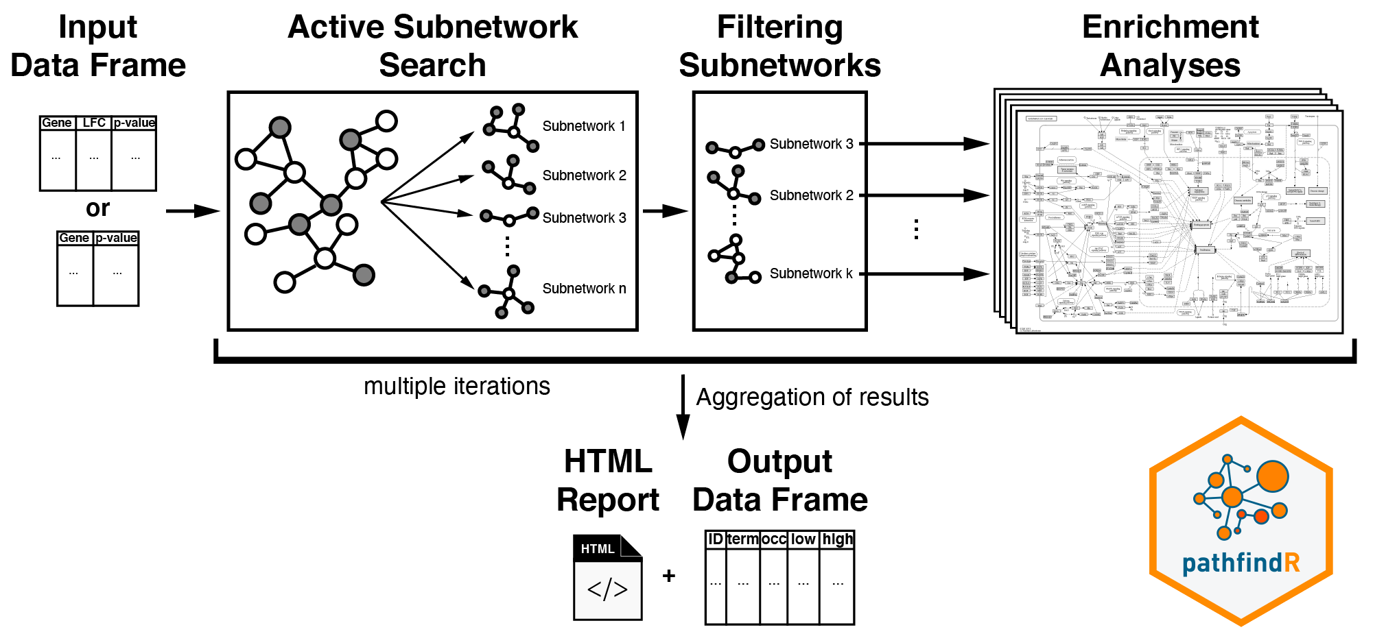
The active-subnetwork-oriented enrichment analysis approach of pathfindR can be summarized as follows: Mapping the input genes with the associated p values onto the PIN (after processing the input), active subnetwork search is performed. The resulting active subnetworks are then filtered based on their scores and the number of significant genes they contain. This filtered list of active subnetworks are then used for enrichment analyses, i.e. using the genes in each of the active subnetworks, the significantly enriched terms (pathways/gene sets) are identified. Enriched terms with adjusted p values larger than the given threshold are discarded and the lowest adjusted p value (over all active subnetworks) for each term is kept. This process of active subnetwork search + enrichment analyses is repeated for a selected number of iterations, performed in parallel. Over all iterations, the lowest and the highest adjusted-p values, as well as number of occurrences over all iterations are reported for each significantly enriched term in the resulting data frame. This active-subnetwork-oriented enrichment approach is demonstrated in the section Active-subnetwork-oriented Enrichment Analysis of this vignette.

The enrichment analysis usually yields a great number of enriched terms whose biological functions are related. Therefore, we implemented two clustering approaches using a pairwise distance matrix based on the kappa statistics between the enriched terms (as proposed by Huang et al. ¹). Based on this distance metric, the user can perform either hierarchical (default) or fuzzy clustering of the enriched terms. Details of clustering and partitioning of enriched terms are presented in the Clustering Enriched Terms section of this vignette.

Other functionality of pathfindR includes:

agglomerated score calculation per each term (to investigate how a gene set is altered in a given sample)
visualization of terms and term-related genes as a graph (to determine the degree of overlap between the enriched terms by identifying shared and/or distinct significant genes) and
pathfindR analysis with custom gene sets are also briefly described.

Active-subnetwork-oriented Enrichment Analysis

For convenience, we provide the wrapper function run_pathfindR() to be used for the active-subnetwork-oriented enrichment analysis. The input for this function must be a data frame consisting of the columns containing: Gene Symbols, Change Values (optional) and p values. The example data frame used in this vignette (example_pathfindR_input) is the dataset containing the differentially-expressed genes for the GEO dataset GSE15573 comparing 18 rheumatoid arthritis (RA) patients versus 15 healthy subjects.

The first 6 rows of the example input data frame are displayed below:

library(pathfindR)
knitr::kable(head(example_pathfindR_input))

Gene.symbol	logFC	adj.P.Val
FAM110A	-0.6939359	0.0000034
RNASE2	1.3535040	0.0000101
S100A8	1.5448338	0.0000347
S100A9	1.0280904	0.0002263
TEX261	-0.3235994	0.0002263
ARHGAP17	-0.6919330	0.0002708

For a detailed step-by-step explanation and an unwrapped demonstration of the active-subnetwork-oriented enrichment analysis, see the vignette Step-by-Step Execution of the pathfindR Enrichment Workflow

Executing the workflow is straightforward (but does typically take several minutes):

output_df <- run_pathfindR(example_pathfindR_input)

Useful arguments

This subsection demonstrates some (selected) useful arguments of run_pathfindR(). For a full list of arguments, see ?run_pathfindR or visit our GitHub wiki.

Filtering Input Genes

By default, run_pathfindR() uses the input genes with p-values < 0.05. To change this threshold, use p_val_threshold:

output_df <- run_pathfindR(example_pathfindR_input, p_val_threshold = 0.01)

Output Directory

By default, run_pathfindR() creates a temporary directory for writing the output files, including active subnetwork search results and a HTML report. To set the output directory, use output_dir:

output_df <- run_pathfindR(example_pathfindR_input, output_dir = "this_is_my_output_directory")

This creates "this_is_my_output_directory" under the current working directory.

In essence, this argument is treated as a path so it can be used to create the output directory anywhere. For example, to create the directory "my_dir" under "~/Desktop" and run the analysis there, you may run:

output_df <- run_pathfindR(example_pathfindR_input, output_dir = "~/Desktop/my_dir")

Note: If the output directory (e.g. "my_dir") already exists, run_pathfindR() creates and works under "my_dir(1)". If that exists also exists, it creates "my_dir(2)" and so on. This was intentionally implemented so that any previous pathfindR results are not overwritten.

Gene Sets for Enrichment

The active-subnetwork-oriented enrichment analyses can be performed on any gene sets (biological pathways, gene ontology terms, transcription factor target genes, miRNA target genes etc.). The available gene sets in pathfindR are “KEGG”, “Reactome”, “BioCarta”, “GO-All”, “GO-BP”, “GO-CC” and “GO-MF” (all for Homo sapiens). For changing the default gene sets for enrichment analysis (hsa KEGG pathways), use the argument gene_sets

output_df <- run_pathfindR(example_pathfindR_input, gene_sets = "GO-MF")

By default, run_pathfindR() filters the gene sets by including only the terms containing at least 10 and at most 300 genes. To change the default behavior, you may change min_gset_size and max_gset_size:

## Including more terms for enrichment analysis
output_df <- run_pathfindR(example_pathfindR_input,
  gene_sets = "GO-MF",
  min_gset_size = 5,
  max_gset_size = 500
)

Note that increasing the number of terms for enrichment analysis may result in significantly longer run time.

If the user prefers to use another gene set source, the gene_sets argument should be set to "Custom" and the custom gene sets (list) and the custom gene set descriptions (named vector) should be supplied via the arguments custom_genes and custom_descriptions, respectively. See ?fetch_gene_set for more details and Analysis with Custom Gene Sets for a simple demonstration.

For details on obtaining organism-specific Gene Sets and PIN data, see the vignette Obtaining PIN and Gene Sets Data.

Filtering Enriched Terms by Adjusted-p Values

By default, run_pathfindR() adjusts the enrichment p values via the “bonferroni” method and filters the enriched terms by adjusted-p value < 0.05. To change this adjustment method and the threshold, set adj_method and enrichment_threshold, respectively:

output_df <- run_pathfindR(example_pathfindR_input,
  adj_method = "fdr",
  enrichment_threshold = 0.01
)

Protein-protein Interaction Network

For the active subnetwork search process, a protein-protein interaction network (PIN) is used. run_pathfindR() maps the input genes onto this PIN and identifies active subnetworks which are then be used for enrichment analyses. To change the default PIN (“Biogrid”), use the pin_name_path argument:

output_df <- run_pathfindR(example_pathfindR_input, pin_name_path = "IntAct")

The pin_name_path argument can be one of “Biogrid”, “STRING”, “GeneMania”, “IntAct”, “KEGG”, “mmu_STRING” or it can be the path to a custom PIN file provided by the user.

# to use an external PIN of your choice
output_df <- run_pathfindR(example_pathfindR_input, pin_name_path = "/path/to/myPIN.sif")

NOTE: the PIN is also used for generating the background genes (in this case, all unique genes in the PIN) during hypergeometric-distribution-based tests in enrichment analyses. Therefore, a large PIN will generally result in better results.

Active Subnetwork Search Method

Currently, there are three algorithms implemented in pathfindR for active subnetwork search: Greedy Algorithm (default, based on Ideker et al. ²), Simulated Annealing Algorithm (based on Ideker et al. ³) and Genetic Algorithm (based on Ozisik et al. ⁴). For a detailed discussion on which algorithm to use see this wiki entry

# for simulated annealing:
output_df <- run_pathfindR(example_pathfindR_input, search_method = "SA")
# for genetic algorithm:
output_df <- run_pathfindR(example_pathfindR_input, search_method = "GA")

Other Arguments

Because the active subnetwork search algorithms are stochastic, run_pathfindR() may be set to iterate the active subnetwork identification and enrichment steps multiple times (by default 1 time). To change this number, set iterations:

output_df <- run_pathfindR(example_pathfindR_input, iterations = 25)

run_pathfindR() uses a parallel loop (using the package foreach) for performing these iterations in parallel. By default, the number of processes to be used is determined automatically. To override, change n_processes:

# if not set, `n_processes` defaults to (number of detected cores - 1)
output_df <- run_pathfindR(example_pathfindR_input, iterations = 5, n_processes = 2)

Output

Enriched Terms Data Frame

run_pathfindR() returns a data frame of enriched terms. Columns are:

ID: ID of the enriched term
Term_Description: Description of the enriched term
Fold_Enrichment: Fold enrichment value for the enriched term (Calculated using ONLY the input genes)
occurrence: The number of iterations that the given term was found to enriched over all iterations
lowest_p: the lowest adjusted-p value of the given term over all iterations
highest_p: the highest adjusted-p value of the given term over all iterations
non_Signif_Snw_Genes (OPTIONAL): the non-significant active subnetwork genes, comma-separated (controlled by list_active_snw_genes, default is FALSE)
Up_regulated: the up-regulated genes (as determined by change value > 0, if the change column was provided) in the input involved in the given term’s gene set, comma-separated. If change column was not provided, all affected input genes are listed here.
Down_regulated: the down-regulated genes (as determined by change value < 0, if the change column was provided) in the input involved in the given term’s gene set, comma-separated

The first 2 rows of the output data frame of the example analysis on the rheumatoid arthritis gene-level differential expression input data (example_pathfindR_input) is shown below:

knitr::kable(head(example_pathfindR_output, 2))

ID	Term_Description	Fold_Enrichment	occurrence	support	lowest_p	highest_p	Up_regulated	Down_regulated
hsa05415	Diabetic cardiomyopathy	3.333277	10	0.0441272	0	0.0000000	NCF4, MMP9, NDUFA1, NDUFB3, UQCRQ, COX6A1, COX7A2, COX7C, GAPDH	ATP2A2, MTOR, PDHA1, PDHB, VDAC1, SLC25A5, PARP1
hsa04130	SNARE interactions in vesicular transport	4.772647	10	0.0142394	0	0.0036008	STX6	STX2, BET1L, SNAP23

By default, run_pathfindR() also produces a graphical summary of enrichment results for top 10 enriched terms, which can also be later produced by enrichment_chart():

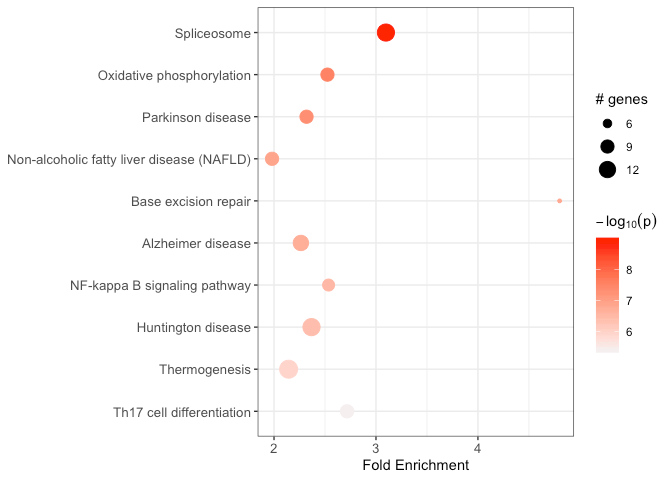
You may also disable plotting this chart by setting plot_enrichment_chart=FALSE and later produce this plot via the function enrichment_chart():

# change number of top terms plotted (default = 10)
enrichment_chart(
  result_df = example_pathfindR_output,
  top_terms = 15
)

HTML Report (created when `output_dir` is set)

The function also creates an HTML report results.html that is saved in the output directory if it’s set. This report contains links to two other HTML files:

1. enriched_terms.html

This document contains the table of the active subnetwork-oriented enrichment results (same as the returned data frame).

2. conversion_table.html

This document contains the table of converted gene symbols. Columns are:

Old Symbol: the original gene symbol
Converted Symbol: the alias symbol that was found in the PIN
Change: the provided change value
p-value: the provided adjusted p value

During input processing, gene symbols that are not in the PIN are identified and excluded. For human genes, if aliases of these missing gene symbols are found in the PIN, these symbols are converted to the corresponding aliases (controlled by the argument convert2alias). This step is performed to best map the input data onto the PIN.

The document contains a second table of genes for which no interactions were identified after checking for alias symbols (so these could not be used during the analysis).

Enriched Term Diagrams

For KEGG enrichment analyses, visualize_terms() can be used to generate KEGG pathway diagrams that are returned as a list of ggraph objects (using ggkegg)::

input_processed <- input_processing(example_pathfindR_input)
gg_list <- visualize_terms(
  result_df = example_pathfindR_output,
  input_processed = input_processed,
  is_KEGG_result = TRUE
)  # this function returns a list of ggraph objects (named by Term ID)

# save one of the plots as PDF image
ggplot2::ggsave(
  "hsa04911_diagram.pdf",   # path to output, format is determined by extension
  gg_list$hsa04911,         # what to plot
  width = 5,                 # adjust width
  height = 5                # adjust height
)

Alternatively (i.e., for other types of non-KEGG enrichment analyses), an interaction diagram per enriched term can be generated again via visualize_terms(). These diagrams are also returned as a list of ggraph objects:

input_processed <- input_processing(example_pathfindR_input)
gg_list <- visualize_terms(
  result_df = example_pathfindR_output,
  input_processed = input_processed,
  is_KEGG_result = FALSE,
  pin_name_path = "Biogrid"
)  # this function returns a list of ggraph objects (named by Term ID)

# save one of the plots as PDF image
ggplot2::ggsave(
  "diabetic_cardiomyopathy_interactions.pdf",   # path to output, format is determined by extension
  gg_list$hsa04911,                             # what to plot
  width = 10,                                    # adjust width
  height = 6                                    # adjust height
)

Clustering Enriched Terms

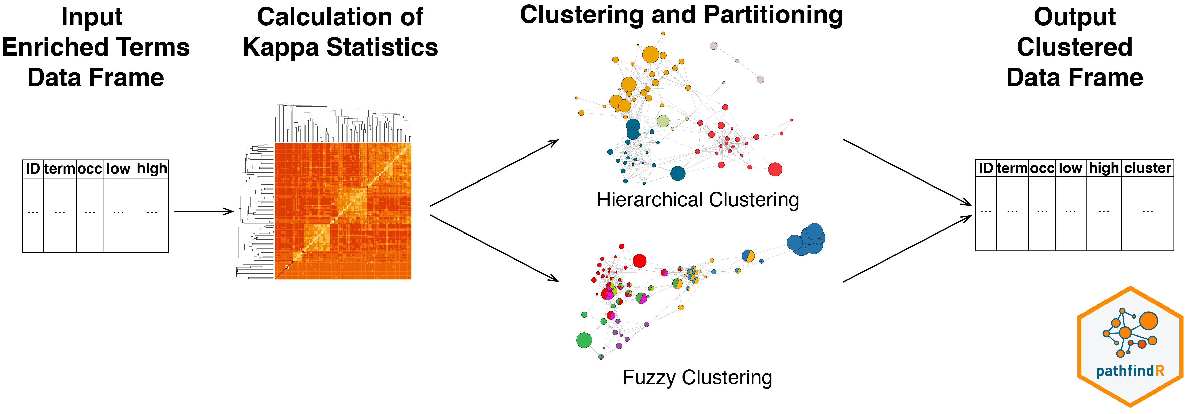
The wrapper function cluster_enriched_terms() can be used to perform clustering of enriched terms and partitioning the terms into biologically-relevant groups. Clustering can be performed either via hierarchical or fuzzy method using the pairwise kappa statistics (a chance-corrected measure of co-occurrence between two sets of categorized data) matrix between all enriched terms.

Hierarchical Clustering

By default, cluster_enriched_terms() performs hierarchical clustering of the terms (using $1 - \kappa$ as the distance metric). Iterating over $2,3,...n$ clusters (where $n$ is the number of terms), cluster_enriched_terms() determines the optimal number of clusters by maximizing the average silhouette width, partitions the data into this optimal number of clusters and returns a data frame with cluster assignments.

example_pathfindR_output_clustered <- cluster_enriched_terms(example_pathfindR_output, plot_dend = FALSE, plot_clusters_graph = FALSE)

## First 2 rows of clustered data frame
knitr::kable(head(example_pathfindR_output_clustered, 2))

	ID	Term_Description	Fold_Enrichment	occurrence	support	lowest_p	highest_p	Up_regulated	Down_regulated	Cluster	Status
1	hsa05415	Diabetic cardiomyopathy	3.333277	10	0.0441272	0	0e+00	NCF4, MMP9, NDUFA1, NDUFB3, UQCRQ, COX6A1, COX7A2, COX7C, GAPDH	ATP2A2, MTOR, PDHA1, PDHB, VDAC1, SLC25A5, PARP1	1	Representative
3	hsa00190	Oxidative phosphorylation	3.003128	10	0.0213591	0	1e-07	NDUFA1, NDUFB3, UQCRQ, COX6A1, COX7A2, COX7C, ATP6V1D, ATP6V0E1	ATP6V0E2	1	Member

## The representative terms
knitr::kable(example_pathfindR_output_clustered[example_pathfindR_output_clustered$Status == "Representative", ])

	ID	Term_Description	Fold_Enrichment	occurrence	support	lowest_p	highest_p	Up_regulated	Down_regulated	Cluster	Status
1	hsa05415	Diabetic cardiomyopathy	3.333277	10	0.0441272	0.0000000	0.0000000	NCF4, MMP9, NDUFA1, NDUFB3, UQCRQ, COX6A1, COX7A2, COX7C, GAPDH	ATP2A2, MTOR, PDHA1, PDHB, VDAC1, SLC25A5, PARP1	1	Representative
2	hsa04130	SNARE interactions in vesicular transport	4.772647	10	0.0142394	0.0000000	0.0036008	STX6	STX2, BET1L, SNAP23	2	Representative
5	hsa04714	Thermogenesis	2.563911	10	0.0274995	0.0000000	0.0000026	NDUFA1, NDUFB3, UQCRQ, COX6A1, COX7A2, COX7C	ADCY7, CREB1, KDM1A, SMARCA4, ACTG1, ACTB, ARID1A, MTOR	3	Representative
9	hsa04921	Oxytocin signaling pathway	2.624956	10	0.0569575	0.0000001	0.0000001	MYL6B, MYL6	EEF2K, EEF2, CALM3, CALM1, NFATC3, ACTG1, ACTB, ADCY7	4	Representative
10	hsa04064	NF-kappa B signaling pathway	3.058201	10	0.0413279	0.0000002	0.0000002	LY96	PRKCQ, CARD11, TICAM1, IKBKB, PARP1, UBE2I, CSNK2A2	5	Representative
11	hsa03040	Spliceosome	3.854831	10	0.0150963	0.0000002	0.0000196	SF3B6, LSM3, BUD31	SNRPB, SF3B2, U2AF2, PUF60, SNU13, DDX23, EIF4A3, HNRNPA1, PCBP1, SRSF8, SRSF5	6	Representative
12	hsa03013	Nucleocytoplasmic transport	3.822751	10	0.0142394	0.0000006	0.0006419	NUP214	RANGAP1, UBE2I, SUMO3, NUP62, NUP93, TNPO1, EIF4A3, RNPS1, SRRM1	7	Representative
18	hsa04141	Protein processing in endoplasmic reticulum	1.458309	10	0.0142394	0.0000165	0.0000165	CKAP4, DDIT3	DDOST, EDEM1, PDIA4, UBE2G1	8	Representative
34	hsa00020	Citrate cycle (TCA cycle)	3.937434	10	0.0137498	0.0001922	0.0013467		MDH2, PDHA1, PDHB	9	Representative
37	hsa04110	Cell cycle	1.550171	10	0.0206246	0.0002953	0.0004008		RBL2, ABL1, HDAC1, CDKN1C, ANAPC1	10	Representative
45	hsa03010	Ribosome	1.837469	10	0.0068749	0.0005741	0.0005741	MRPS18C, RPS24, MRPL33, RPL26, RPL31, RPL39	RPLP2	11	Representative
46	hsa03050	Proteasome	1.749971	10	0.0075481	0.0006684	0.0018936		PSMD7, PSMB10	12	Representative
50	hsa03022	Basal transcription factors	4.374927	4	0.0056694	0.0008495	0.0059660	GTF2B, GTF2H5	TAF1L, TAF4, TAF15	13	Representative
67	hsa03460	Fanconi anemia pathway	2.410674	7	0.0062893	0.0034174	0.0034174		TELO2, MLH1, RPA1	14	Representative
89	hsa00330	Arginine and proline metabolism	4.921793	7	0.0062893	0.0157779	0.0469727	ARG1	CKB, ALDH9A1, CNDP2, PYCR2, GOT1	15	Representative
100	hsa00062	Fatty acid elongation	3.423856	1	0.0055249	0.0244440	0.0244440		HADH, ECHS1	16	Representative
107	hsa03060	Protein export	1.789743	3	0.0055249	0.0300181	0.0300181		SRP54	17	Representative

After clustering, you may again plot the summary enrichment chart and display the enriched terms by clusters:

# plotting only selected clusters for better visualization
selected_clusters <- subset(example_pathfindR_output_clustered, Cluster %in% 5:7)
enrichment_chart(selected_clusters, plot_by_cluster = TRUE)
#> Plotting the enrichment bubble chart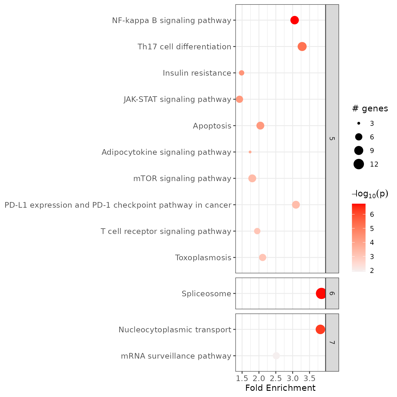

For details, see ?hierarchical_term_clustering

Heuristic Fuzzy Multiple-linkage Partitioning

Alternatively, the fuzzy clustering method (as described by Huang et al.⁵) can be used:

clustered_fuzzy <- cluster_enriched_terms(example_pathfindR_output, method = "fuzzy")

For details, see ?fuzzy_term_clustering

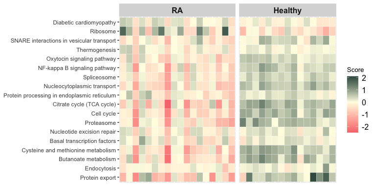
Aggregated Term Scores per Sample

The function score_terms() can be used to calculate the agglomerated z score of each enriched term per sample. This allows the user to individually examine the scores and infer how a term is overall altered (activated or repressed) in a given sample or a group of samples.

## Vector of "Case" IDs
cases <- c(
  "GSM389703", "GSM389704", "GSM389706", "GSM389708",
  "GSM389711", "GSM389714", "GSM389716", "GSM389717",
  "GSM389719", "GSM389721", "GSM389722", "GSM389724",
  "GSM389726", "GSM389727", "GSM389730", "GSM389731",
  "GSM389733", "GSM389735"
)

## Calculate scores for representative terms
## and plot heat map using term descriptions
representative_df <- example_pathfindR_output_clustered[example_pathfindR_output_clustered$Status == "Representative", ]
score_matrix <- score_terms(
  enrichment_table = representative_df,
  exp_mat = example_experiment_matrix,
  cases = cases,
  use_description = TRUE, # default FALSE
  label_samples = FALSE, # default = TRUE
  case_title = "RA", # default = "Case"
  control_title = "Healthy", # default = "Control"
  low = "#f7797d", # default = "green"
  mid = "#fffde4", # default = "black"
  high = "#1f4037" # default = "red"
)

Comparison of 2 pathfindR Results

The function combine_pathfindR_results() allows combination of two pathfindR active-subnetwork-oriented enrichment analysis results for investigating common and distinct terms between the groups. Below is an example for comparing results using two different rheumatoid arthritis-related data sets(example_pathfindR_output and example_comparison_output).

combined_df <- combine_pathfindR_results(
  result_A = example_pathfindR_output,
  result_B = example_comparison_output,
  plot_common = FALSE
)
#> You may run `combined_results_graph()` to create visualizations of combined term-gene graphs of selected terms

For more details, see the vignette Comparing Two pathfindR Results

Analysis with Custom Gene Sets

As of v1.5, pathfindR offers utility functions for obtaining organism-specific PIN data and organism-specific gene sets data via get_pin_file() and get_gene_sets_list(), respectively. See the vignette Obtaining PIN and Gene Sets Data for detailed information on how to gather PIN and gene sets data (for any organism of your choice) for use with pathfindR.

It is possible to use run_pathfindR() with custom gene sets (including gene sets for non-Homo-sapiens species). Here, we provide an example application of active-subnetwork-oriented enrichment analysis of the target genes of two transcription factors.

We first load and prepare the gene sets:

## CREB target genes
CREB_target_genes <- normalizePath(system.file("extdata/CREB.txt", package = "pathfindR"))
CREB_target_genes <- readLines(CREB_target_genes)[-c(1, 2)] # skip the first two lines

## MYC target genes
MYC_target_genes <- normalizePath(system.file("extdata/MYC.txt", package = "pathfindR"))
MYC_target_genes <- readLines(MYC_target_genes)[-c(1, 2)] # skip the first two lines

## Prep for use
custom_genes <- list(TF1 = CREB_target_genes, TF2 = MYC_target_genes)
custom_descriptions <- c(TF1 = "CREB target genes", TF2 = "MYC target genes")

We next prepare the example input data frame. Because of the way we choose genes, we expect significant enrichment for MYC targets (40 MYC target genes + 10 CREB target genes). Because this is only an example, we also assign each genes random p-values between 0.001 and 0.05.

set.seed(123)

## Select 40 random genes from MYC gene sets and 10 from CREB gene sets
selected_genes <- sample(MYC_target_genes, 40)
selected_genes <- c(
  selected_genes,
  sample(CREB_target_genes, 10)
)

## Assign random p value between 0.001 and 0.05 for each selected gene
rand_p_vals <- sample(seq(0.001, 0.05, length.out = 5),
  size = length(selected_genes),
  replace = TRUE
)

example_pathfindR_input <- data.frame(
  Gene_symbol = selected_genes,
  p_val = rand_p_vals
)
knitr::kable(head(example_pathfindR_input))

Gene_symbol	p_val
HNRNPD	0.01325
IL1RAPL1	0.00100
CD3EAP	0.00100
LTBR	0.02550
CGREF1	0.00100
TPM2	0.05000

Finally, we perform active-subnetwork-oriented enrichment analysis via run_pathfindR() using the custom genes as the gene sets:

example_custom_genesets_result <- run_pathfindR(
  example_pathfindR_input,
  gene_sets = "Custom",
  custom_genes = custom_genes,
  custom_descriptions = custom_descriptions,
  min_gset_size = 1,   # do not limit the gene set size for demo
  max_gset_size = Inf, # do not limit the gene set size for demo
)

knitr::kable(example_custom_genesets_result)

ID	Term_Description	Fold_Enrichment	occurrence	support	lowest_p	highest_p	Up_regulated	Down_regulated
TF2	MYC target genes	18.61325	1	0.9435484	0.00e+00	0.00e+00	ACVR2B, ADAMTS19, ARL3, BEX1, C9orf139, CCDC6, CEP57, CNNM1, CNPY3, COL25A1, DEPDC7, DZIP1, EBNA1BP2, EIF3A, ELOVL5, FAM117A, FKBP5, HPCA, HSP90AB1, KCNQ5, KLF11, LCLAT1, MMP23B, MNT, NEK6, OPRD1, PFN1, POGK, REEP3, SAMD12, SLC24A4, SMC3, TBL1X, TESK2, TFB2M, TIMM8A, USP2, WDR77, XPO5, ZBTB11, ZCWPW1
TF1	CREB target genes	21.08612	1	0.2177419	1.16e-05	1.16e-05	ADAP1, ELOVL5, HAS1, HSP90AB1, ID1, NOL4, PLK4, PNMA3, SCAMP5, SNAP25, ZBTB11, ZNF687

It is also possible to run pathfindR using non-human organism annotation. See the vignette pathfindR Analysis for non-Homo-sapiens organisms

Huang DW, Sherman BT, Tan Q, et al. The DAVID Gene Functional Classification Tool: a novel biological module-centric algorithm to functionally analyze large gene lists. Genome Biol. 2007;8(9):R183.↩︎
Ideker T, Ozier O, Schwikowski B, Siegel AF. Discovering regulatory and signalling circuits in molecular interaction networks. Bioinformatics. 2002;18 Suppl 1:S233-40.↩︎
Ideker T, Ozier O, Schwikowski B, Siegel AF. Discovering regulatory and signalling circuits in molecular interaction networks. Bioinformatics. 2002;18 Suppl 1:S233-40.↩︎
Ozisik O, Bakir-Gungor B, Diri B, Sezerman OU. Active Subnetwork GA: A Two Stage Genetic Algorithm Approach to Active Subnetwork Search. Current Bioinformatics. 2017; 12(4):320-8. /1574893611666160527100444↩︎
Huang DW, Sherman BT, Tan Q, et al. The DAVID Gene Functional Classification Tool: a novel biological module-centric algorithm to functionally analyze large gene lists. Genome Biol. 2007;8(9):R183.↩︎

Ege Ulgen

2025-02-17

Overview

Active-subnetwork-oriented Enrichment Analysis

Useful arguments

Filtering Input Genes

Output Directory

Gene Sets for Enrichment

Filtering Enriched Terms by Adjusted-p Values

Protein-protein Interaction Network

Active Subnetwork Search Method

Other Arguments

Output

Enriched Terms Data Frame

HTML Report (created when `output_dir` is set)

Enriched Term Diagrams

Clustering Enriched Terms

Hierarchical Clustering

Heuristic Fuzzy Multiple-linkage Partitioning

Aggregated Term Scores per Sample

Comparison of 2 pathfindR Results

Analysis with Custom Gene Sets

Introduction to pathfindR

Ege Ulgen

2025-02-17

Overview

Active-subnetwork-oriented Enrichment Analysis

Useful arguments

Filtering Input Genes

Output Directory

Gene Sets for Enrichment

Filtering Enriched Terms by Adjusted-p Values

Protein-protein Interaction Network

Active Subnetwork Search Method

Other Arguments

Output

Enriched Terms Data Frame

HTML Report (created when output_dir is set)

Enriched Term Diagrams

Clustering Enriched Terms

Hierarchical Clustering

Heuristic Fuzzy Multiple-linkage Partitioning

Aggregated Term Scores per Sample

Comparison of 2 pathfindR Results

Analysis with Custom Gene Sets

HTML Report (created when `output_dir` is set)